Getting Unique Values Only

Often times when you are working with Excel, you want to reduce a list of items so that only the unique instances are listed. In other words, if, within a column or list an item happens to be duplicated, you want that item to appear only once. Maybe you have a mailing list, for example, and fear that some customers may be entered more than once. Or perhaps you’ve been collecting emails and are now ready to send out promotional or “Thank you” emails, but don’t want to spam people with multiple messages.

Luckily, Excel makes it very easy to do this, saving you from yourself. In fact, there are two ways. One is simpler and built in to Excel’s multiple functionalities. The other is a bit more difficult and less intuitive, but is more flexible and dynamic. I explain them both to give you flexibility in dealing with these types of business problems. For my example, I use a simple list of animals where a couple of them (cat, bird) are each repeated.

Note: This tip is for Excel 2007, but is applicable, with a tweak or two, with other versions of Excel.

Method 1:

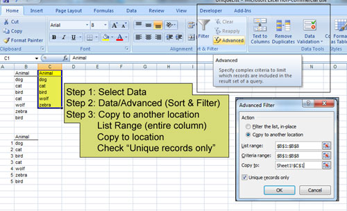
1. Select data from which you want to retrieve only the unique values. Underline, or otherwise differentiate, the header so that Excel can recognize it as such.
2. Under the “Data” Ribbon, select the “Advanced” Option.
3. Under Action, select “Copy to another location.”
4. The “List Range” should be populated with the data set selected in Step 1
5. Choose the same range for the “Criteria Range” (I normally copy and paste) from above (the “List Range”)
6. Check the box next to “Unique Records”
7. Hit the “OK” button

Excel provides an easy way to get the Unique Values from a list

Method 2:

1. To the left of the first item on the list (not the header), enter the number 1
2. To the left of the second item on the list, enter:

   =IF(COUNTIF($B$2:B3,B3)=1,A2+1,A2)
   where:

   1. A2 is the cell containing the number 1 from Step 1
   2. $B$2:B3 is a dynamic (moving) range that will increase for each row, moving down from the current row

   What this formula does is count how many times the current item in the list has occurred so far, including the current row. If the count is one, it increases the count by one, treating the item as a unique value. If the count is more than one, the current item is treated as a duplicate and the number does not increase.

3. Copy (or fill) down the formula from Step 2 to the row containing the last item in the list.
4. To the right of the first tem on the list, enter:

   =IFERROR(VLOOKUP(ROWS($B$2:B2),$A$2:$B$8,2,0),””)
   where:

   1. $B$2:B2 is a dynamic (moving) range that will increase for each row, moving down from the current row
   2. Rows($B$2:B2) is 1, but as the formula is copied down, becomes, 2 (for Rows($B$2:B3), 3 (for Rows($B$2:B4), etc.
   3. $A$2:$B$8 is the range, two columns, including the one created Step 2

   What this formula does is, by way of VLOOKUP, check the first column (A) in the range $A$2:$B$8 for the value resulting from the function Rows($B$2:B2). Again, this will result in 1, 2, 3, etc. (for as many rows as you copy or fill down). Once the formula finds the first instance of that number, it will stop. It then returns the value in the same row from the 2^nd column. Finally, the “0”, which is almost always used, tells the vlookup formula to return an exact match, not the closest value. The IFERROR() function is wrapped around the VLOOKUP, used to replace any errors (#N/A) returned by the VLOOKUP function (after the last unique value has been found) with a blank.

5. Copy (or fill) down the formula from Step 4 to the row containing the last item in the list.