Data Validation: Part 2 of 3

Using named ranges is a very useful trick and can be applied in a lot of ways, including data validation.

In part one of this Data Validation series, I showed you how simple it is to add validation to your spreadsheets, increasing the ease and accuracy of data entry. In that post, I showed two ways of limiting the allowed values for any particular cell. The most straightforward method involves entering the values directly into the source box. Alternatively, you can enter the allowed values in a column somewhere else on the spreadsheet and then refer to that range of cells in the validation window. The downside to this method is that you must list the values on the same spreadsheet as the field on which you are applying validation, adding unnecessary clutter. Of course you could hide the column or put the values well off of the visible screen (e.g. column ZZ or something like that), but you’d have to unhide the column or scroll over to the far right of the spreadsheet every time you wanted to update the list. That is obviously not ideal.

Indirect Function: using named range as the source.

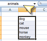
You can simplify things by applying a few simple techniques. While the “Source” box on the data validation window doesn’t allow a range outside of the current worksheet, it does allow named ranges, which can refer to these external ranges. To do so, however, requires the use of the Indirect Function, which will treat anything you feed it as if you’d typed it directly. While typing “animals” into the “Source” box will create a drop down list of one value- “animals”, for example, using Indirect(“animals”) will create a drop down box with the values of the named range called “animals.”

Specifically, apply the following steps to use this method:

1. On a separate worksheet (which you can later hide if you wish), enter the values you wish to allow
2. Name the range by using one of the following methods:
   1. Under Formulas Ribbon, choose “Name Manager”; then create “new”
   2. Select the range containing the values; in the address bar, type the desired name; in our example, we use “animals”
3. On the “Data Tools” Ribbon, select Data Validation/Data Validation; the “Data Validation” window will appear
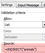
4. On the “Validation Criteria” tab, select “List” under for the “Allow” option
5. The “Source” box will now be active; in type:

   =INDIRECT(“animals”)

6. Hit the “Ok” button

It’s that simple. In part three of this series, I’ll show you another cool trick. What if you wanted to restrict allowable values in a cell based on the value in another field? For example, let’s say you have a field for “State.” Depending upon the value in that cell, you then want to allow a finite list of cities to be selected. Again, with the use of named ranges and the Indirect function, this is a lot easier than you might think.