The Bluford Principle

The windshield keeps you focused on where you are going, but the rear view mirror reminds you where you came from.

We spend Christmas Eve every year at my in-laws in Modesto, CA, a little over an hour drive from my hometown of San Jose. We always have a great time there during the Holidays. My children get to see and spend time with their cousins, whom they don’t see very often. My wife gets to hang out with her siblings, whom because of life’s commitments- kids and work just to name a couple- she also sees a lot less than she probably should. And I get a mini-vacation, a few days that, because there are more adult eyes to look after ours and the other children, I get to relax and unwind a little.

As the stoplight turned green and we proceeded through the last busy intersection on the final stretch of road before my in-laws’ home, I noticed a man standing in a used car lot, which because it was nearly nine pm on Christmas Eve, had been closed for several hours. He was bundled up next to a streetlight, smoking what I’d hoped was a cigarette. “Look at that man,” my daughter said. “He must be cold,” my son added. Upon hearing my children, my eyes immediately glanced at the temperature gauge in my car. It read 36 degrees. Those readers who reside in the Northeast, or even the Midwest or South for that matter, might not see a man standing in 36 degree weather as particularly alarming. For a California boy, though, witnessing this man standing alone, on a street corner, in almost freezing weather, on Christmas Eve no less; was a perfect opportunity to empty my bucket (referring to the great book, How Full Is Your Bucket? If you have children and haven’t shared with them the kid version of this wonderful book, you definitely need to pick it up) and also teach my kids a valuable lesson.

It sounds so simple. “Appreciate what you have.” We make it poetic at times. “Be sure to smell the roses.” And sometimes it’s beaten over our heads by our moms. “Boy, there are people in Africa that wish they had half of what you have!” (That last one is courtesy of my mom, bless her soul.) But the truth is we all- or at least most of us- suffer from this affliction. The problem, I’ve determined, is not that we are all ingrates, as my wife hilariously proclaims at times. The issue is that it’s hard to feel that way–grateful and thankful– while working from a model or view of the world built on ill-advised and unproductive reference and comparison. I’ve gone so far as to name it. I call it the Bluford Principle. Why the Bluford Principle? Well, mostly because I haven’t heard anyone else refer to this dilemma, on which I’ll elaborate in a moment, in quite this way. And maybe a little because I just like the way it sounds. Read more of this post

Data Validation: Part 3 of 3

Make your spreadsheets stand out with Data Validation and Dependent Drop-Down Lists

In part one of this Data Validation series, I showed you how simple it is to add validation to your spreadsheets, increasing the ease and accuracy of data entry. In that post, I showed two ways of limiting the allowed values for any particular cell. The most straightforward method involves entering the values directly into the source box. Alternatively, you can enter the allowed values in a column somewhere else on the spreadsheet and then refer to that range of cells in the validation window. The downside to this method is that you must list the values on the same spreadsheet as the field on which you are applying validation, adding unnecessary clutter. Of course, as I mentioned, you could hide the column or put the values well off of the visible screen (e.g. column ZZ or something like that), but you’d have to unhide the column or scroll over to the far right of the spreadsheet every time you wanted to update the list. That is obviously not ideal.

A better way to accomplish this was discussed in part two of this Data Validation Series, where I showed how using a named range allows for a cleaner worksheet. I showed how listing the values you want to allow for a specific cell (field) on another sheet, then naming this range so that you can refer to it in the Data Validation window is cleaner and more efficient than listing them in the Data Validation window itself or separately in a list, but on the same sheet. Read more of this post

Data Validation: Part 2a of 3

Convert your named Range into a Table for more flexibility

In part 2 of this Data Validation Series, I showed how using a named range when adding data validation to your fields allows for a cleaner worksheet. Listing the values you want to allow for a specific cell (field) on another sheet, then naming this range so that you can refer to it in the Data Validation window, I showed you, is more efficient and cleaner than listing them in the Data Validation window itself or separately in a list, but on the same sheet.

But we can enhance this method even further. Using the named range, you might have discovered, makes adding an item to the list difficult. You either have to change the referenced range area each time you add an item or you have to make the original range large enough to include further inclusions. Unfortunately, creating a range with blank rows leaves spaces in your data validation list.  That’s obviously not ideal or neat.

A great workaround for this is to convert the range of allowable values into a table as follows: Read more of this post

Data Validation: Part 2 of 3

Using named ranges is a very useful trick and can be applied in a lot of ways, including data validation.

In part one of this Data Validation series, I showed you how simple it is to add validation to your spreadsheets, increasing the ease and accuracy of data entry. In that post, I showed two ways of limiting the allowed values for any particular cell. The most straightforward method involves entering the values directly into the source box. Alternatively, you can enter the allowed values in a column somewhere else on the spreadsheet and then refer to that range of cells in the validation window. The downside to this method is that you must list the values on the same spreadsheet as the field on which you are applying validation, adding unnecessary clutter. Of course you could hide the column or put the values well off of the visible screen (e.g. column ZZ or something like that), but you’d have to unhide the column or scroll over to the far right of the spreadsheet every time you wanted to update the list. That is obviously not ideal.

Indirect Function: using named range as the source.

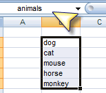
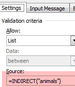
You can simplify things by applying a few simple techniques. While the “Source” box on the data validation window doesn’t allow a range outside of the current worksheet, it does allow named ranges, which can refer to these external ranges. To do so, however, requires the use of the Indirect Function, which will treat anything you feed it as if you’d typed it directly. While typing “animals” into the “Source” box will create a drop down list of one value- “animals”, for example, using Indirect(“animals”) will create a drop down box with the values of the named range called “animals.”

Specifically, apply the following steps to use this method:

  1. On a separate worksheet (which you can later hide if you wish), enter the values you wish to allow
  2. Name the range by using one of the following methods:
    1. Under Formulas Ribbon, choose “Name Manager”; then create “new”
    2. Select the range containing the values; in the address bar, type the desired name; in our example, we use “animals”
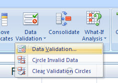
  3. On the “Data Tools” Ribbon, select Data Validation/Data Validation; the “Data Validation” window will appear
  4. On the “Validation Criteria” tab, select “List” under for the “Allow” option
  5. The “Source” box will now be active; in type:

    =INDIRECT(“animals”)

  6. Hit the “Ok” button

It’s that simple. In part three of this series, I’ll show you another cool trick. What if you wanted to restrict allowable values in a cell based on the value in another field? For example, let’s say you have a field for “State.” Depending upon the value in that cell, you then want to allow a finite list of cities to be selected. Again, with the use of named ranges and the Indirect function, this is a lot easier than you might think.

Data Validation: Part 1 of 3

Get familiar with the Data Validation Ribbon; it can save you from headaches due to errors in data entry.

If you work with data often, and especially if you collaborate or share your information and work with others, you know this to be fact: like my kids when they tell me they are going to sleep when I know they’re not; if left unsupervised, your colleagues will undoubtedly screw up your spreadsheet. Of course that is partly poking fun, but you get the point and can certainly relate. One of the biggest problems I’ve confronted over the years working with data has to be maintaining accurate and easy data entry.

Fortunately, the two–accuracy and simplicity– go hand in hand. Making the process simple by reducing the potential for human error is paramount. This cannot be understated and serves two purposes. As mentioned in one of my favorite books, The E-Myth Revisited by Michael E. Gerber, one of the biggest mistakes people in business make is making the success of their company, department, or group too heavily dependent on smart people and excellent workers. While I certainly understand the importance of a good team, something that revealed itself time and time again while playing sports my entire life, I also know that having a great structure and process that allows players or employees of different types and skills to succeed, is as important and effective. Making the structure of the “program” simple and effective is step one. Once that is accomplished, communicating that structure clearly and explicitly so that those charged with carrying out the plan will be successful is step two and a natural extension of step one.

The Data Validation Window allows you to customize data entry, user communication, and error handling.

In the working world, this theory manifests itself in many ways. One small way is in the countless reports, processes, and other forms of communications we all share between and amongst each other. Within that context, Data Validation in Microsoft Excel can be an extremely helpful tool. Instead of allowing free and manual entry, I am of the mindset that whenever possible you should restrict the possibilities people have and, therefore, probability of error. Not only does this ensure accurate information is collected and shared. But it also allows employees to perform their jobs well, thus enjoying them more, and frees them up to perform more important duties and grow professionally in business-critical areas.

It’s really pretty simple. To make sure data is entered correctly, apply data validation to a cell, by doing the following:

  1. Select the cell on which you’d like to apply validation
  2. On the “Data Tools” Ribbon, select Data Validation/Data Validation; the “Data Validation” window will appear
  3. There are three tabs on the “Data Validation” pop-up
    1. Settings: Under ‘Validation Criteria’, select “List” for the “Allow:” option
      1. The “Source:” box will then appear. You can either type in the options, separated by a comma; or enter a range of cells that contains the list of values you allow.
    2. Input Message: Allows you to enter text that appears when the cell with validation is selected
    3. Error Message: Allows you to customize the message that appears if invalid data is entered
  4. Using a range on your spreadsheet to limit values is great, but hiding them from the user is even better. I'll show you how in Part II.

    Select OK

Very simple, right? Well, what if you want to use a range for the list, but don’t want it to appear on the same sheet, cluttering up things. In part two of this series, I’ll show you a trick for that.