Named Ranges

If you’re like me, your spreadsheets can become rather unwieldy.  More often than not, a big reason is that I have to refer to a cell in several places.  While using absolute references and relative references appropriately is helpful, they don’t make things as easy as they could be.

Figure 1: Sales Data Table

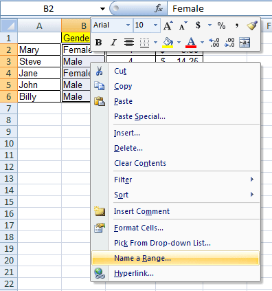
Say you’re working with the table on the right.  You have been asked to report the  Total males and total females, as well as the total items and dollars sold for each gender

Using the Countif() and Sumif() formulas, the most common ways would be:

for the total person for each gender:
=COUNTIF(B2:B6,”Male”) (the count for female is exactly the same)

for the sum of items sold and dollars collected:
=SUMIF(B2:B6,”Male”,C2:C6) (the sum for females and/or Total Dollars collected is exactly the same)

But if you ever wanted to go back and check to see what you were trying to accomplish with the formulas, it might take some time before you remember. You can make things easier by using named ranges.  So:

Figure 2: Named Range Creation

Instead of B2:B6, you could write “GenderCol” for the column titled Gender; you could do the same for the “ItemsSold” (ItemsSold instead of C2:C6) and TotalDols (TotalDollars instead of D2:D6).

To make it work, simply highlight the range of cells you’d like to name; then, right-click and select “name a range”.  Name your range in the next window and you’re ready to go.

Now, instead of using the column letter(s) and row number(s), you can use the range name.

For example:

=SUMIF(GenderCol,”Male”,C2:C6)

Wasn’t that easy?

Again, you can do the same for the other columns in this example, defining the Total Items Sold and Total Dollars Collected columns.