Custom Number Format

Figure 1: Write Functions max, min, and average

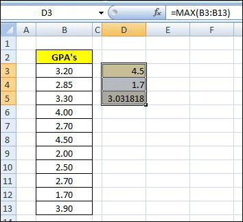
Do you ever want to include additional information inside of a cell that contains or calculates a number?  Here’s how.  Let’s pretend you have a classroom of students.  You have a list of their Semester Grade Point Averages and want to quickly summarize the class, looking at the highest, lowest, and average.

To accomplish it, you write the formulas to calculate the three figures.  The three functions you’ll use are:
max (), min (), and average () [See Figure 1: Write Functions: max, min, and average]

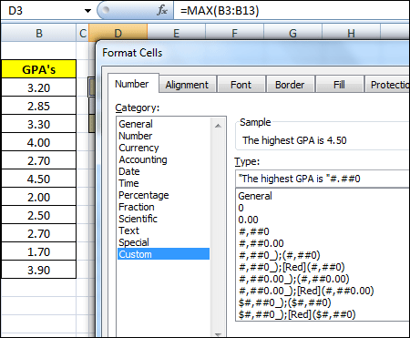
The next step is to reformat the cell, changing the default or current setting.  Right click on the cell, and select “Format Cells” toward the bottom of the drop-down window.  Once selected, the first tab of the format window, “Number”, will appear.  Choose the “Custom” Category at the bottom.

You’ll then see (to the right) a “Sample” section which shows the result of any custom function you write based on the selected cell’s current contents.  There are several predefined choices, but we’ll write our own.  We can, however, look at this list to get an idea of the different number and date characters (#,$,mm,yyyy) allowed.

Figure 2: Changing the Cell Number Format

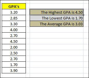
First, we put the text that we’d like to appear in the field regardless of its contents.  This is done by placing the desired text inside of double quotes (“”).  We follow that with the format we’d like for our number.  In this case we have one number, followed by a “.”, then two decimal places of numbers.  The result, again, is shown in the ‘Example’ box. [See Figure 2: Changing the Cell Number Format]  Work on the custom format until everything looks right, then click “OK”.  And you’re done! Open Example

Figure 3: Final Output