Hiding your work- Part 1

What if you want to hide your work?

There are times when you are working on a spreadsheet, when you must create placeholders. Perhaps you are applying some custom formatting to a specific area, but must reference information in another sheet. (For more information on Custom Formatting, see Custom Formatting). You’ll quickly discover that Excel doesn’t allow you to do that. Or maybe you are modeling your business and want to refer to a different sheet and perform different calculations when the month in question is closed and you have actual data than when it is in the future and you are forecasting. An easy way to tell Excel where to look is to put an “A” (for actual) or “F” (for forecast) in the top row. (How you get Excel to automatically determine which to use can be done in a number of different ways, but some functions you might use INDEX, VLOOKUP, IF, or MAX functions; I’ll be sure to fit in a discussion of each of those at some point.)

But you don’t necessarily want the user of the spreadsheet to see this work, right?  Well, you can hide it in one of several ways. You could change the font color to white (the same color as the background), but any user who selected that and other cells, would still see the cell contents. You could hide the section (row and/or column) that contains the information. Again, though, a savvy user could simply unhide the areas you’ve tried to conceal. Or you could put the information in a cell or cells far enough out of reach where no user would think to look. In Excel 2007, for example, you could put the information in row 1048576, column XFD (absolute bottom, far, far right). But that, too, seems silly.

Luckily, there is a pretty simple solution. With custom formatting, which I covered briefly in a previous post on custom number formatting, you can simply tell Excel to show nothing. Yup, it’s that easy. Here’s what you do:

Hide- but don't CHANGE- a cell's contents

1. Select Cell or Cells whose contents you’d like to hide
   1. Right Click and select ‘Format Cells’ or
   2. Use the Ctrl-1 Shortcut to bring up the ‘Format Cells’ Window
2. Select “Number” tab
3. Choose “Custom” under Category

   Quick Note/Tutorial: Custom formatting syntax is broken into four parts, each normally separated by a “;”

   1. How you want positive numbers displayed
   2. How you want negative numbers displayed
   3. How you want 0 (zero) values displayed
   4. What you want displayed if the cell contains text
4. In the formatting box (right below “Type:”), type two semicolons (“;;”)
5. THAT’S IT!

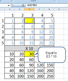
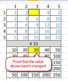
Remember that, although the user cannot see the cell’s contents, the spreadsheet is not impacted (i.e. the cell doesn’t change). You can still work with it the same way you would any other cell. See attached HidingInfo as an example.

I’ve also included a brief video to explain this process.  Please enjoy.