It’s Absolute(ly) Relative

If I had a dollar for every time someone asked me “what the heck are those dollar signs for?,” I’d be a millionaire.  Well, anyone worth their weight in gold as an Excel user should really understand what those pesky dollar signs are used for.

Most of us know how to use relative references

It’s really pretty simple.  The inclusion of dollar signs ($) in a formula changes at least part of the cell reference from relative to absolute.  Let me explain.  You see, Microsoft Excel is a very, very powerful tool. So powerful, in fact, that more times than not, it tries to help you get your work done faster and more effectively, even attempting to save you, the user, from yourself.  Like auto-numbering and spell-check in Microsoft Word, this type of “help” is what we’ve come to expect with Microsoft products.  So when you copy a formula for use somewhere else in your worksheet, which I’m sure you’ve done, Excel assumes that you want to keep the same relationship.

For example, say if you have three columns of data that represent daily transactions for your store.  Column A represents quantity sold, Column B lists the price per item, and Column C is the product of the two (A*B).  Because of this intuitiveness built into Excel, you need only enter “=A2*B2” into column C (assuming the first row is your column headings).  You can then copy and paste or fill-down the formula. And, as I’m sure you know, Excel will continue with the relative positions (A3*B3, A4*B4, etc.).

Nothing changes when you use $Absolute$References

But that is not always helpful and, if you happen to miss this error (for example, you don’t get an error result or the result doesn’t stick out like a sore thumb), it can even cause serious problems.

So, what are some formulas where this relative positioning might not work?  Here are some examples:

1. You are working with data in which you are searching another table to retrieve further information.  If you are using a vlookup, for example, and the table being searched is in the range D5:F30, then copying the formula would move the table being searched around.  If you copied and pasted “=vlookup(“dog”,D5:F30,2,0)” into a cell right below the current location, the result would be: “=vlookup(“dog”,D6:F31,2,0)”.  Similarly incorrect, if you copied and pasted the same formula into the cell directly to the right, the resulting formula would be: “=vlookup(“dog”,E5:G30,2,0)”.  Both of these are obviously changing where and how the formula will look up data.
2. What if you are working with a table of Commissions due for your Sales People.  In two columns, you have the name of the Sales Person and his or her Total Sales.  If everyone in Sales receives the same commission percentage, you have this rate listed in one cell.  (Note: doing things this way also allows for quick changing.  If management decides to increase the commission percentage, it need only be changed in one location.)  But back to the relative versus absolute issue.  If you have the commission percentage listed in one cell and want to multiply that by the sales generated for each employee, you simply multiply the first employee’s sales by this cell.  But you cannot simply copy and paste this formula down the column.  That’s because Excel will assume, without telling it otherwise, that you want the cells that you are multiplying to move one cell down, as well.  For the Sales part of the formula, that’s perfectly fine.  Not for the commission percentage, though, because that figure is, and in the formula should remain, static.

There are three types of Formula References: Relative, Absolute, and Mixed.  Relative references assume that, when copying the formula elsewhere, you want the relationships among the cells to which the formula is referring to change their positioning, keeping the same relationship.  These types of references are most typical and don’t require any dollar signs (A1).  Absolute references tell Excel the opposite, that you don’t want the referenced cell to change at all.  In these cases, you’d put a “$” in front of both the column and the row portion of the cell reference ($A$1).  And finally, Mixed references mean you want only part of the formula– either the column ($A1) or the row (A$1)– to be locked, or fixed.

You can fix the row (or column) only

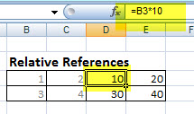
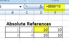
To further illustrate, let’s say you have a 2×2 grid.  Staring with the upper left-hand corner (let’s call this cell A1) and working clockwise, the figures in the cells are 1,2,4, and 3.  You’d like to multiply the figure in each cell by 10, creating a new 2×2 grid directly adjacent and to the right.  If in the upper left-hand corner of the new table, you multiply 10 by cell A1, the result (in C1) will be 10 (10*1).  You can then copy and paste the formula into the other three boxes, and the results will be 20, 40, and 30.  (See Attached: Absolute_v_Relative_References).   If instead of A1, you used $A$1, all of the four cells will be 10 (1*10).  The tricky part is when only part of the cell reference is absolute.  If, for example, we used $A1, the results, clockwise, will be 10, 10, 30, and 30.  Because we are locking the first column, we never use the 2 or the 4 in our formulas.  And if we used A$1, the results would be 10, 20, 20, 10.  This is because now the row is locked, so we never use the 3 or the 4.

Now that example is obscure and doesn’t help much.  So let’s look at a real-world application.  What if you have data showing daily sales made by representatives in one of four regions: West, North, South, and East.  You’d like to create a dynamic table that automatically calculates total sales for every month/region combination.  Using the very versatile SUMPRODUCT function, which I’ve covered in a few other posts, we can search the data pretty easily. But to be able to create the formula once, then copy it, we must adhere to three key rules:

1. First, since we are searching specific data ranges (e.g. the columns containing the sales date {to make sure it matches the current month/year}), we must keep that range fixed, or absolute.
2. Since the month labels are all in the same row, we must make sure that the portion of the formula referring to the month is fixed
3. Since the region labels are all in the same column, we must make sure that the portion of the formula referring to the region is fixed

When done properly, copying and pasting is a breeze!

Again, please see the attached to gain a further understanding.  If anything is confusing or you have further questions, please don’t hesitate to ask.