What quarter is it?

When you’re working with financial data (forecasts, revenue or sales targets, financials), you are certainly used to working at the annual and monthly level.  And doing so, whether with a spreadsheet or accounting software, is straightforward.  Grouping by quarter, though, is not as simple, at least when working in Excel.  But, as we accounting and finance people learn, it can be the most useful.  Monthly information often represents too small a slice of data to offer any useful insight- at least in its own context.  On the other hand, while annual information gives you a much better feel for what’s going on with the business, it happens too infrequently to allow management or ownership to do anyting about it.

It makes sense, then, to organize and analyze important information by quarter.  After all, there’s a reason big companies report these results to all who are listening. Read more of this post
Hiding your work- Part 1

What if you want to hide your work?

There are times when you are working on a spreadsheet, when you must create placeholders. Perhaps you are applying some custom formatting to a specific area, but must reference information in another sheet. (For more information on Custom Formatting, see Custom Formatting). You’ll quickly discover that Excel doesn’t allow you to do that. Or maybe you are modeling your business and want to refer to a different sheet and perform different calculations when the month in question is closed and you have actual data than when it is in the future and you are forecasting. An easy way to tell Excel where to look is to put an “A” (for actual) or “F” (for forecast) in the top row. (How you get Excel to automatically determine which to use can be done in a number of different ways, but some functions you might use INDEX, VLOOKUP, IF, or MAX functions; I’ll be sure to fit in a discussion of each of those at some point.)

But you don’t necessarily want the user of the spreadsheet to see this work, right?  Well, you can hide it in one of several ways. You could change the font color to white (the same color as the background), but any user who selected that and other cells, would still see the cell contents. Read more of this post

It’s Absolute(ly) Relative

If I had a dollar for every time someone asked me “what the heck are those dollar signs for?,” I’d be a millionaire.  Well, anyone worth their weight in gold as an Excel user should really understand what those pesky dollar signs are used for.

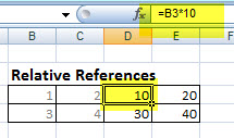
Most of us know how to use relative references

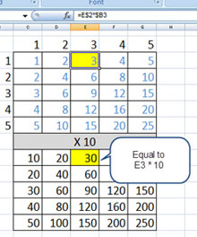
It’s really pretty simple.  The inclusion of dollar signs ($) in a formula changes at least part of the cell reference from relative to absolute.  Let me explain.  You see, Microsoft Excel is a very, very powerful tool. So powerful, in fact, that more times than not, it tries to help you get your work done faster and more effectively, even attempting to save you, the user, from yourself.  Like auto-numbering and spell-check in Microsoft Word, this type of “help” is what we’ve come to expect with Microsoft products.  So when you copy a formula for use somewhere else in your worksheet, which I’m sure you’ve done, Excel assumes that you want to keep the same relationship.

For example, say if you have three columns of data that represent daily transactions for your store.  Column A represents quantity sold, Column B lists the price per item, and Column C is the product of the two (A*B).  Because of this intuitiveness built into Excel, you need only enter “=A2*B2” into column C (assuming the first row is your column headings).  You can then copy and paste or fill-down the formula. And, as I’m sure you know, Excel will continue with the relative positions (A3*B3, A4*B4, etc.). Read more of this post

Easy way to get the last day of the month in Excel

There are a lot of times I need to get the last day of a particular month.  One example I’ve used lately is trying to forecast sales for the remainder of a month using the average to date.  If it’s February 12, for instance, and the average daily sales so far are 12k.  I want to extrapolate that out for the rest of the month.  To do so, I need for Excel to know how many more days are remaining in the month- February.

Excel makes this very easy in one of two ways: Read more of this post

Floor and Ceiling Functions

While the ROUNDUP (round up to the nearest number, specifying the number of digits), ROUNDDOWN (round down to the nearest number, specifying the number of digits), and ROUND (round to nearest number up or down, specifying the number of digits) are very helpful, sometimes you wish to round up or down to a specific multiple.  Maybe you are dealing with large numbers and want to deal work only with multiples of 1,000 or 10,000.  Or maybe you’re building a graph or chart and want to minimize the scale.  The best way to do that, you decide, is to make the base (lower bound value) lower than, but as close to, the lowest number as possible.

No matter the reason, performing this is easy.  For each of them, you only need the number you are rounding and the multiple you’d like to round (up or down) to.  Examples follow:

Value: A1=1,798

Floor(A1,5)=1,795
Floor(A1,10)=1,790
Floor(A1,25)=1,775
Floor(A1,100)=1,700
Floor(A1,1,000)=1,000
Floor(A1,1,500)=1,500
Floor(A1,2,000)=0

Ceiling(A1,5)=1,800
Ceiling(A1,10)=1,800
Ceiling(A1,25)=1,800
Ceiling(A1,100)=1,800
Ceiling(A1,1,000)=2,000
Ceiling(A1,1,500)=3,000
Floor(A1,2,000)=0

As always, if you have questions, drop me a line or post a comment.